I’ve been doing research that shows change in opinion over time across the electoral cycle and I wanted to visualize primary elections - but there’s a whole lot of them. Rather than copying them down by hand, I decided to scrape them from a PDF. I’ve included the full code to reproduce what I did below.
Now, you might notice that the document in question is pretty short and you could probably copy and paste this thing. My main interest here was to use this as a toy example to show how scraping structured data from a document like this could be done. Hopefully it’s useful as a reference, even if it’s a little overkill for this specific instance. This code scales pretty well to a document of any size.
Note: see the Tools section below for links to more info on what’s going on here
In R, a good tool for this is tabulizer, a wrapper for a library of Java tools (Tabula).
First, keep in mind: this package is just a way for you to use R to talk to Java. I don’t do Java myself and ran into a few wonky errors. See below for a little more detail in case you run into them1
I installed from the github repo using devtools (you’ll need to install devtools first, if you haven’t already):
devtools::install_github(c("ropenscilabs/tabulizerjars", "ropenscilabs/tabulizer"), args = "--no-multiarch")
# Load in packages

library(tidyverse)
## ── Attaching packages ────────────────────────────────── tidyverse 1.2.1 ──## ✔ ggplot2 2.2.1 ✔ purrr 0.2.4
## ✔ tibble 1.3.4 ✔ dplyr 0.7.4
## ✔ tidyr 0.7.2 ✔ stringr 1.2.0
## ✔ readr 1.1.1 ✔ forcats 0.2.0## ── Conflicts ───────────────────────────────────── tidyverse_conflicts() ──
## ✖ dplyr::filter() masks stats::filter()
## ✖ dplyr::lag() masks stats::lag()library(stringr)
library(tabulizer)
library(purrr)The FEC has election dates posted as PDFs. You could probably scrape these from Wikipedia or something similar, but I like to go straight to the source.
prim_loc <- 'https://transition.fec.gov/pubrec/2008pdates.pdf'

prim <- extract_tables(prim_loc)
It might take a minute. Now you’ve got all the data stored in a useful R object - a list where each top-level element is a page of the PDF.
str(prim)## List of 6
## $ : chr [1:41, 1:5] "STATE" "" "" "" ...
## $ : chr [1:40, 1:5] "STATE" "" "" "" ...
## $ : chr [1:46, 1:6] "STATE" "" "" "" ...
## $ : chr [1:29, 1:6] "STATE" "" "" "" ...
## $ : chr [1:47, 1:7] "STATE" "" "" "Iowa" ...
## $ : chr [1:36, 1:7] "STATE" "" "" "D.C." ...Let’s look at the first page. If you look into the first element, it’s stored as a two dimensional character vector - rows and columns extracted from that page.
str(prim[[1]])## chr [1:41, 1:5] "STATE" "" "" "" "Alabama" "Alaska" ...prim[[1]][c(1:20), ]## [,1] [,2] [,3]
## [1,] "STATE" "PRESIDENTIAL" "PRESIDENTIAL"
## [2,] "" "PRIMARY" "CAUCUS DATE"
## [3,] "" "DATE" ""
## [4,] "" "" ""
## [5,] "Alabama" "2/5" ""
## [6,] "Alaska" "" "2/5"
## [7,] "American Samoa" "" "2/23 (Republicans)"
## [8,] "" "" "2/5 (Democrats)"
## [9,] "Arizona" "2/5" ""
## [10,] "Arkansas" "2/5" ""
## [11,] "California" "" ""
## [12,] "" "2/5" ""
## [13,] "Colorado" "" "2/5"
## [14,] "Connecticut" "2/5" ""
## [15,] "Delaware" "2/5" ""
## [16,] "" "" ""
## [17,] "D.C." "2/12" ""
## [18,] "Florida" "1/29" ""
## [19,] "Georgia" "2/5" ""
## [20,] "Guam" "" "3/8 (Republicans)"
## [,4] [,5]
## [1,] "FILING" "INDEPENDENT 1"
## [2,] "DEADLINE FOR" "FILING DEADLINE"
## [3,] "PRIMARY" "FOR GENERAL"
## [4,] "BALLOT ACCESS" "ELECTION"
## [5,] "11/7" "9/6"
## [6,] "n/a" "8/6"
## [7,] "n/a" "n/a"
## [8,] "" ""
## [9,] "12/17 5pm" "6/4 5pm"
## [10,] "11/19 Noon" "8/4"
## [11,] "12/4 (Democrats)" ""
## [12,] "11/23 (Other Parties)" "8/8"
## [13,] "n/a" "6/17 3pm"
## [14,] "12/17 4pm" "8/6"
## [15,] "12/10" "7/25 (Independent)"
## [16,] "" "9/1 (Third/Minor)"
## [17,] "12/14 5pm" "8/27"
## [18,] "10/31" "7/15"
## [19,] "11/1" "7/15"
## [20,] "n/a" "n/a"Let’s just slice off the stuff we need. First drop the pages we don’t need (the pages are redundant, the actual primary data shown in alpha order are on pages 1 and 2). Second, we don’t care about the filing deadlines, so lets just keep the first three columns (with states and dates). Third, let’s drop those headers (the first four rows) and keep everything else.
I make them into actual data.frames (well, tibbles) so we can use other dplyr verbs on them. Then to combine all list elements into one big table and give them useful variable names.
prim_df<-
prim %>%
.[1:2] %>%
map(., `[`, c(-1:-4), c(1:3) ) %>%
map(as.tibble) %>%
bind_rows() %>%
set_names(c("state", "primary", "caucus") ) %>%

na_if("") %>%
filter(!(is.na(state) & is.na(primary) & is.na(caucus)))

head(prim_df)
## # A tibble: 6 x 3
## state primary caucus
## <chr> <chr> <chr>
## 1 Alabama 2/5 <NA>
## 2 Alaska <NA> 2/5
## 3 American Samoa <NA> 2/23 (Republicans)
## 4 <NA> <NA> 2/5 (Democrats)
## 5 Arizona 2/5 <NA>
## 6 Arkansas 2/5 <NA>tail(prim_df)## # A tibble: 6 x 3
## state primary caucus
## <chr> <chr> <chr>
## 1 <NA> <NA> 4/5 (Republicans)
## 2 Washington 2/19 2/9
## 3 West Virginia 5/13 <NA>
## 4 Wisconsin 2/19 <NA>
## 5 Wyoming <NA> 1/5 (Republicans)
## 6 <NA> <NA> 3/8 (Democrats)Note two things: 1) First, I used backticks around the subset operator to apply it as a function [ . 2) map comes from purrr. Rather than using the apply() set of functions in base R, (or the ply family frm the earlier plyr package) as with other languages, map lets me apply a function across elements of a vector and returns that vector object. So in this case, I get back a list with the top four rows removed, retaining the first three columns.
Now some general cleanup: For empty strings, make them NA and get rid of rows where everything’s empty. Now fill in states where there’s an implied value that isn’t included in the PDF.
prim_df<-
prim_df %>%
fill(state)

head(prim_df)
## # A tibble: 6 x 3
## state primary caucus
## <chr> <chr> <chr>
## 1 Alabama 2/5 <NA>
## 2 Alaska <NA> 2/5
## 3 American Samoa <NA> 2/23 (Republicans)
## 4 American Samoa <NA> 2/5 (Democrats)
## 5 Arizona 2/5 <NA>
## 6 Arkansas 2/5 <NA>tail(prim_df)## # A tibble: 6 x 3
## state primary caucus
## <chr> <chr> <chr>
## 1 Virgin Islands <NA> 4/5 (Republicans)
## 2 Washington 2/19 2/9
## 3 West Virginia 5/13 <NA>
## 4 Wisconsin 2/19 <NA>
## 5 Wyoming <NA> 1/5 (Republicans)
## 6 Wyoming <NA> 3/8 (Democrats)A couple spot revisions…
prim_df$caucus[prim_df$caucus == '1/25-2/7'] <- '1/25-2/7 (Republicans)'
prim_df$caucus[prim_df$caucus == '(Republicans)'] <- NA
Now, rather than a wide format with a column for each type of election, let’s make just one row per election and get rid of those where there’s no date value.
primary_dates_2008 <-
prim_df %>%
gather('primary', 'caucus', key = 'elex_type', value = 'date') %>%
filter(!(is.na(date)))

head(primary_dates_2008)
## # A tibble: 6 x 3
## state elex_type date
## <chr> <chr> <chr>
## 1 Alabama primary 2/5
## 2 Arizona primary 2/5
## 3 Arkansas primary 2/5
## 4 California primary 2/5
## 5 Connecticut primary 2/5
## 6 Delaware primary 2/5tail(primary_dates_2008)## # A tibble: 6 x 3
## state elex_type date
## <chr> <chr> <chr>
## 1 Puerto Rico caucus 2/24 (Republicans)
## 2 Virgin Islands caucus 2/9 (Democrats)
## 3 Virgin Islands caucus 4/5 (Republicans)
## 4 Washington caucus 2/9
## 5 Wyoming caucus 1/5 (Republicans)
## 6 Wyoming caucus 3/8 (Democrats)Finally, separate the date and the party labels into separate columns and format the dates with some regular expressions.
library(lubridate)##
## Attaching package: 'lubridate'## The following object is masked from 'package:base':
##
## dateprimary_dates_2008 <-
primary_dates_2008 %>%
mutate(
elex_party = str_extract(date, regex("[a-zA-Z]+")),
date = str_extract(date, regex("\\d+/\\d+")) %>%
paste0("/2008") %>%
mdy()
)
head(primary_dates_2008)## # A tibble: 6 x 4
## state elex_type date elex_party
## <chr> <chr> <date> <chr>
## 1 Alabama primary 2008-02-05 <NA>
## 2 Arizona primary 2008-02-05 <NA>
## 3 Arkansas primary 2008-02-05 <NA>
## 4 California primary 2008-02-05 <NA>
## 5 Connecticut primary 2008-02-05 <NA>
## 6 Delaware primary 2008-02-05 <NA>tail(primary_dates_2008)## # A tibble: 6 x 4
## state elex_type date elex_party
## <chr> <chr> <date> <chr>
## 1 Puerto Rico caucus 2008-02-24 Republicans
## 2 Virgin Islands caucus 2008-02-09 Democrats
## 3 Virgin Islands caucus 2008-04-05 Republicans
## 4 Washington caucus 2008-02-09 <NA>
## 5 Wyoming caucus 2008-01-05 Republicans
## 6 Wyoming caucus 2008-03-08 DemocratsHere’s a quick-and-dirty plot just to check to see this all makes sense:
library(ggplot2)

ggplot() +
  geom_text(data= primary_dates_2008, aes(x = date, y=0, label = state, color=coalesce(elex_party, 'Both'), angle=90), size=3, position=position_jitter(width=2,height=8), alpha=0.6) +
  scale_color_manual(values = c("black", "blue","red"), drop=F) +
  theme_minimal() +
  guides(color=guide_legend(title="Election Type")) +
  labs(x = "", y = "", title = "Primary dates across 2008 election cycle") +
  theme(panel.background = element_rect(fill = "white", colour = "white"), axis.text.y=element_blank()) +
  scale_x_date(date_labels = "%b %Y")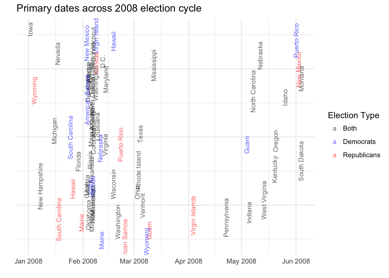
Yeah, this looks about right: Iowa and New Hampshire at the front; a giant jumble around Super Tuesday and lots of dead space in the middle of spring.
Tools:
A few links to tutorials on the functions I use above
purr: map
dplyr: filter, mutate, gather, bind_rows, na_if, fill
maggritr: %>%, set_names
stringr: str_replace, str_extract, etc
Some coding concepts:
Regular expressions: Introduction and cheatsheet
`[`: Advanced R > Functions. See ‘Infix functions’
Apparently a lot of folks have trouble using R packages that have a Java dependency - or getting them to work with RStudio, if that’s how you do your work. This is too bad, because there’s a lot of utility you can get out of them.
A brief summary of some of what I’ve found in dealing with this: You need to have the Java runtime environment installed first before doing any of this. Simple enough. But sometimes the R packages and the environments where they run have trouble finding the right libraries to get R and Java to talk to each other. In the case of using RStudio, I found a solution that involved 1) installing rJava first, 2) from terminal, enteringR CMD javarecogto find out where the libraries in question were being stored and 3) calling them directly in R before loading the tabulizer package. In my case that’s:dyn.load('/Library/Java/JavaVirtualMachines/jdk1.8.0_144.jdk/Contents/Home/jre/lib/server/libjvm.dylib')If you’re running on a Mac, odds are you’ll just need to replace thejdk1.8.0_144.jdkpart with whatever JDK version you’ve installed - and javarecog should tell you what you need to know.↩